
Corsica Predictions Explained
Anyone who has attempted it will attest that predicting hockey games is not easy. Being able to beat the odds set by sportsbooks like Pinnacle and Bovada is harder still. Nevertheless, with the right combination of skill, smarts and luck, one can have success betting on the NHL. We exercised every last ounce of our expertise and left no datum unturned in this endeavor.
We targeted three types of betting lines: the Money Line, the Puck Line (Spread) and the Over/Under.
Money Line
The Money Line simply gives odds on either team winning the game in regulation, overtime or the shootout. This is the simplest type of problem to solve, but that doesn’t necessarily make it easy.
Take the following example:
CAR +144 @ FLA -160
Here, Florida is both the home team and the favourite, as indicated by the negative odds. A Money Line of -160 means you would have to wager $160 to win $100 in addition to your original wager. Conversely, you would stand to win $144 on $100 wagered on Carolina (the underdog). Using some quick arithmetic, we can convert these odds to implied probabilities:
So,
Note that the implied probabilities do not sum to 100%. This is called Vigorish or Vig, and it tilts the scale in favour of the oddsmaker regardless of the outcome. In the above example, the true probability of a win would have to exceed 61.53% in order to reliably profit from repeated plays on Florida to win. Similarly, the true win probability would need to surpass 40.98% for a positive expected value on Carolina to win.
Hence, we want to develop a method of producing win probabilities and we strive to come nearer to the theoretical “true probability” than the implied odds. We formulate the problem as follows:
Given an arbitrarily large set of parameters relating to a game to be played between a Home Team and an Away Team, what is the probability that the Home Team will win in regulation, overtime or the shootout?
and we use accuracy and log-loss to measure model efficacy, where a higher accuracy and lower log-loss is better. For context, a naïve model that simply uses the average home team win probability produces an accuracy of 54.79% and a log-loss of 0.6886 while the “de-juiced” implied odds from Bovada score an accuracy of 58.30% and a log-loss of 0.6736.
There are countless ways one can approach this problem. What we found was that the optimal results came not from selecting the best model, but from combining these various models. This concept is known as stacking or ensemble learning. It has been found that stacking performs better in practice when its components are not highly correlated. In accordance with this principle, we set out to create sub-models that were both diverse and yet individually strong predictors.
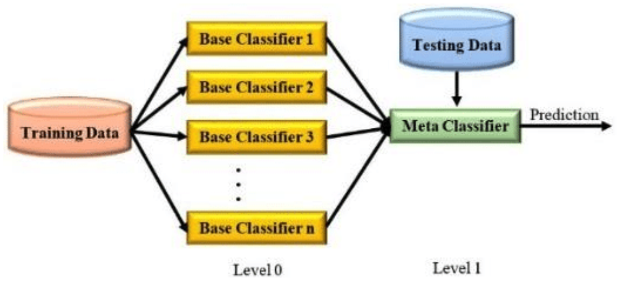
In total, 14 different sub-models were used in the ensemble. Furthermore, many of these sub-models employ bagging or boosting, making them ensembles themselves. Among these sub-models is Salad, a previous attempt at this problem which itself is an ensemble of 11 models. The end result is an ensemble of ensembles – many models working in unison towards a common end.
To promote diversity in these various components, several feature sets were produced containing different variable groups. Features were selected according to their importance as computed by the CatBoost algorithm. Among the most important features were:
- Strength of forwards/defence as reported by the mean Player Rating of the starting lineup
- The K Rating of home and away teams
- The Adjusted 5-on-5 Fenwick differential of home and away teams in recent games
- The Elo rating of home and away teams
Additionally, special data arrays were created for consumption by the two Convolution Neural Networks. One of these accepts a 2×20 matrix representing the roster alignment of both teams with values equal to the Player Rating belonging to the roster member at each position.
Players are ranked in decreasing order of their total Time On Ice in the previous 5 games played. The expectation was that a convolutional network could uncover complex relationships within the matching between rosters and potential imbalances between kernels.
The second array contains head-to-head features. That is, for each i from 1 to n, the ith column of the mxn matrix contains a pair of competing or opposing values. For example, one such pair is the home team’s GF/60 rate and the away team’s GA/60 rate. This head-to-head pair matches one team’s offence to the other’s defence. The motivation in creating such a structure was to accelerate or ease the process of uncovering such relationships by the neural network.
The remaining feature sets ranged in size between 8 and several thousand statistics. The larger feature sets were used for residual boosting where the aim was to issue increasingly moderate corrections to the output of a previous model. This approach was used in one case to adjust the implied odds given by Bovada. Given a training set of Money Line odds and known outcomes, we can construct a model targeting the residuals from the implied probabilities – the error margins themselves. Thus, by adding this new model’s output to the implied probability, we hope to decrease this error. Formally:
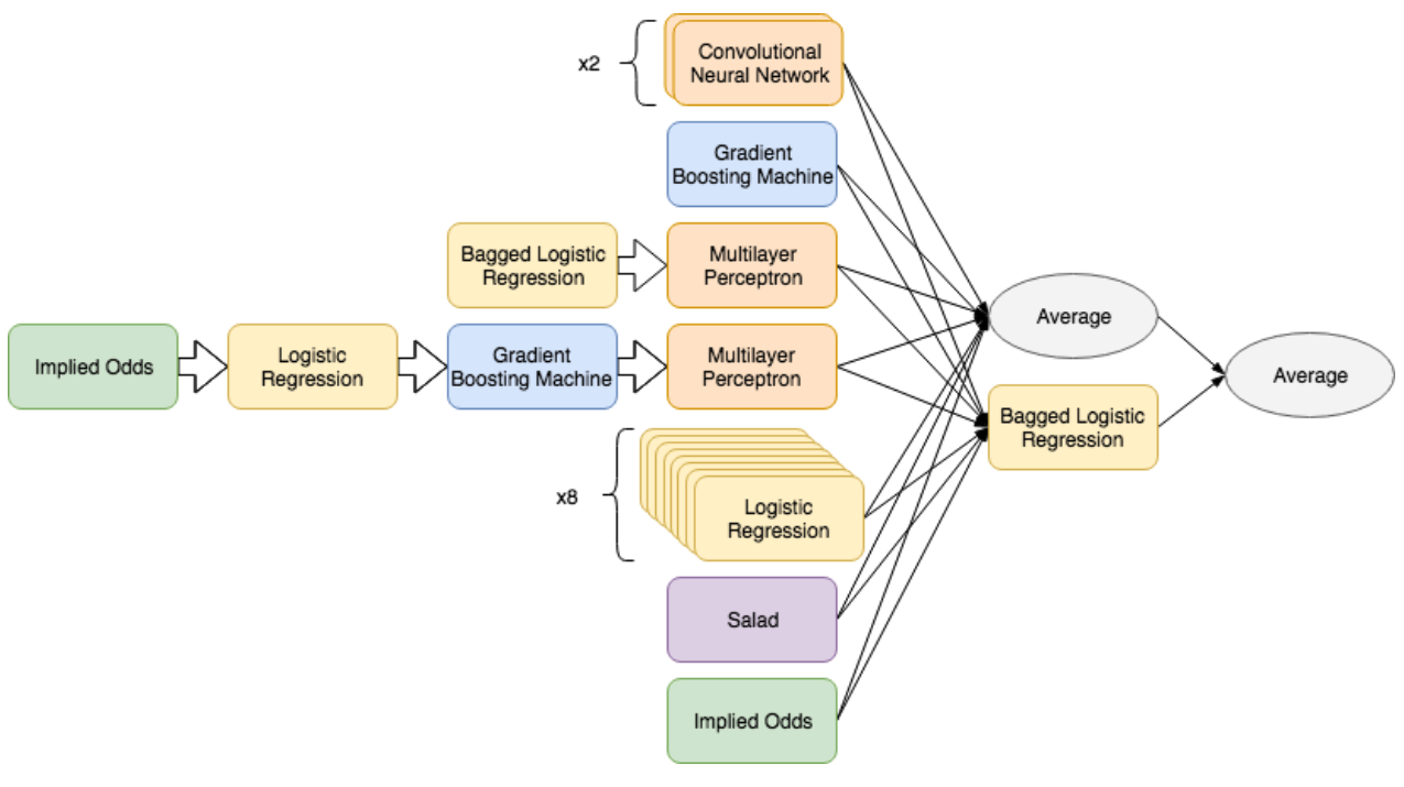
Interestingly, we can build a sequence of such boosting models by setting h(x) to h(x) + g(x) and repeating the steps as many times as desired. In our case, we performed 3 rounds of boosting: first with a simple logistic regression model and limited variables, then a gradient-boosted decision trees model with an increased number of variables (~1000), and finally a heavily regularized neural network with yet more variables (~2500). This series of corrections improved the out-of-sample log-loss from Bovada’s odds from 0.6710 to 0.6693.
A bagged logistic regression model was used to combine outputs from these sub-models and its result was subsequently averaged with the average of the first layer outputs. This two-step ensemble procedure is an attempt to regularize the final predictions, which are prone to overconfidence when generated by committee from a set of sub-models known to perform well on a given data set. The inclusion of the de-juiced implied Bovada probabilities can be seen as a type of hedging.
Each sub-model underwent a two-step validation and testing suite. First, a rolling forecast origin validation was performed using the 2013-14, 2014-15, 2015-16 and 2016-17 seasons. Each of these seasons was held out once as a testing fold and all the previous seasons served to train a model that would subsequently produce predictions on the held-out season. The 4 folds were combined and used to calculate accuracy and log-loss. Model tuning was performed to the end of minimizing this reported log-loss. Once such a model had been
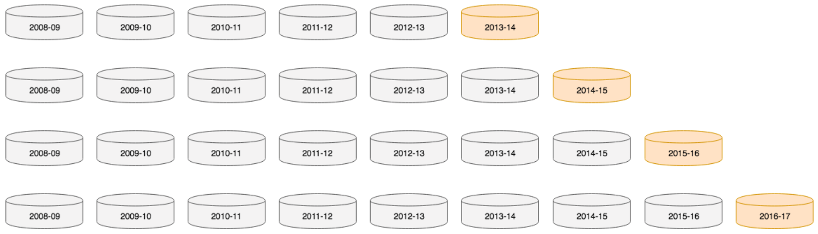
finalized, it was tested on the 2017-18 season, which had heretofore been kept hidden. In the case of the ensemble, a validation data set first had to be created from out-of-sample sub-model predictions. This first layer was produced in the same manner the sub-models were validated – by predicting each of the seasons between 2013-14 and 2016-17 using a model trained on all previous seasons. Ensembles were then tested on this 4-season data set using random k-fold cross-validation. Below is a summary of validation and test scores obtained from each sub-model and the final ensemble:
| Model Description | Validation Log-Loss | Validation Accuracy | Testing Log-Loss | Testing Accuracy |
|---|---|---|---|---|
| CNN 1 | 0.6754139 | 0.5784091 | 0.6753460 | 0.5900350 |
| CNN 2 | 0.6742186 | 0.5804924 | 0.6762582 | 0.5917832 |
| CatBoost 1 | 0.6725936 | 0.5825758 | 0.6727148 | 0.5847902 |
| Logistic + MLP | 0.6731487 | 0.5878788 | 0.6725045 | 0.5900350 |
| Boosted Odds | 0.6692580 | 0.5986880 | 0.6734504 | 0.5839161 |
| Logistic 1 | 0.6736301 | 0.5789773 | 0.6753663 | 0.5821678 |
| Logistic 2 | 0.6734568 | 0.5816288 | 0.6727997 | 0.5865385 |
| Logistic 3 | 0.6705773 | 0.5916667 | 0.6703581 | 0.6031469 |
| Logistic 4 | 0.6705278 | 0.5882576 | 0.6683209 | 0.5970280 |
| Logistic 5 | 0.6769002 | 0.5732955 | 0.6736581 | 0.5900350 |
| Logistic 6 | 0.6783505 | 0.5721591 | 0.6790032 | 0.5882867 |
| Logistic 7 | 0.6740068 | 0.5767045 | 0.6750339 | 0.5882867 |
| Logistic 8 | 0.6794484 | 0.5638258 | 0.6835999 | 0.5743007 |
| Implied Odds | 0.6712447 | 0.5893939 | 0.6700579 | 0.5952797 |
| Salad | 0.6675118 | 0.5886364 | 0.6712618 | 0.5847902 |
| Average | 0.6710315 | 0.5915417 | 0.6716220 | 0.5926573 |
| Ensemble | 0.6687927 | 0.5962500 | 0.6703090 | 0.5900350 |
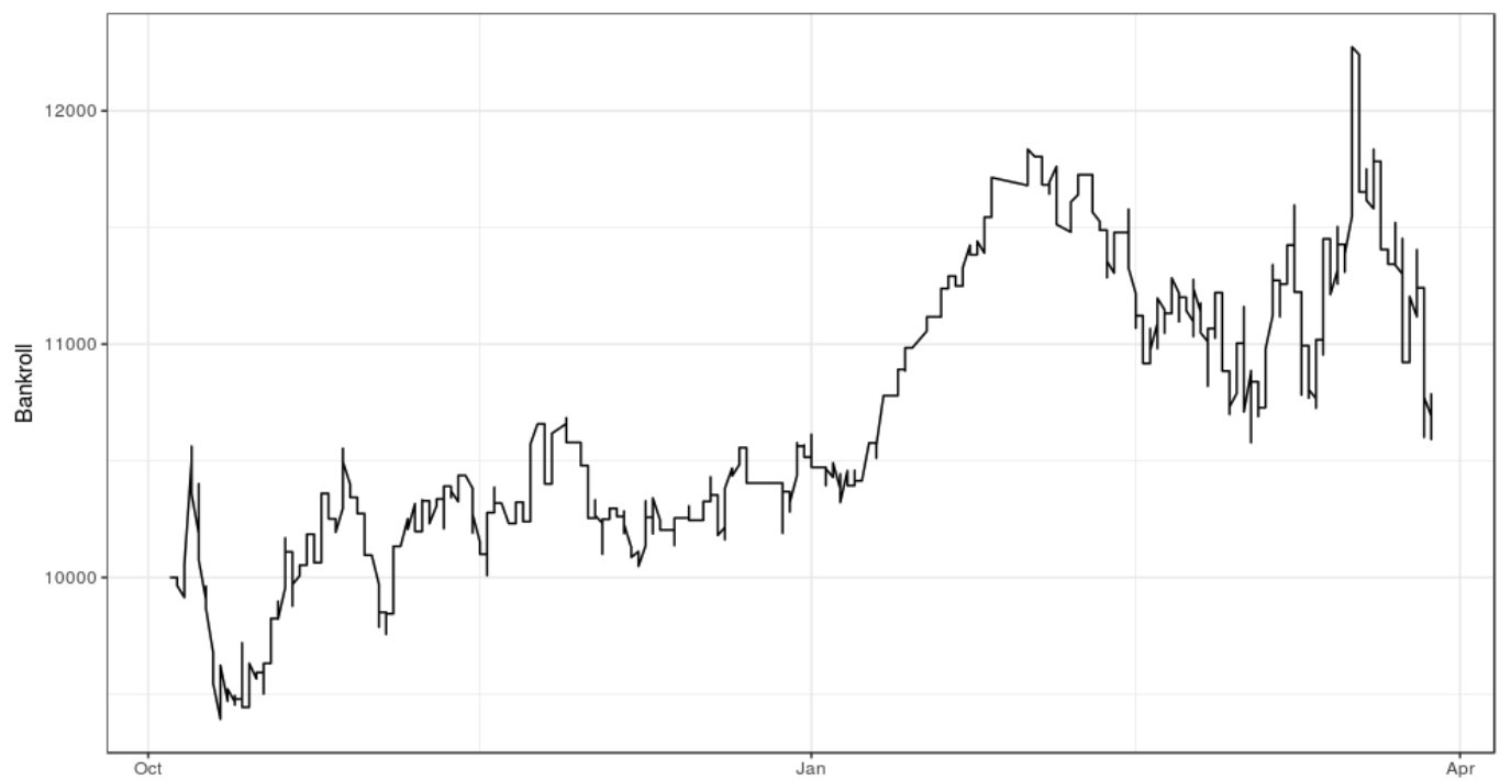
The ensemble performed slightly worse than Salad in terms of log-loss in validation, but did significantly better on accuracy. We believe this new ensemble will generally perform better on new data and this belief is substantiated by its results on the final testing set. Despite the fact this model did not outperform the Bovada implied odds in terms of log-loss within the testing sample, back-testing indicates profit would have been generated during the 2017-18 season using a relatively simple betting strategy. The reported earnings against the Bovada closing Money Line were 7.9 units, with a ROI of 2.16%.
Over/Under
While an Over/Under bet can be approached as a binary problem if the given goal total is known, it is preferred to build a framework capable of producing over/under probabilities for any arbitrary total. With this in mind, we decided to formulate this bet type as a multiclassification problem, where a likelihood is sought for each possible outcome. Thus, probabilities can be summed on either side of a given over/under total. Because there is no theoretical limit to the quantity of goals that can be scored in an NHL game, we imposed an artificial limit of 17 – the most recorded in our database.
A two-step process was used to predict these goal totals, the first of which was to predict the number of goals scored by either team. This problem necessitated a similar approach to what would ultimately be used for game totals. That is, a model was trained capable of generating probabilities for each possible team-goal output. Here, we impose a limit of 12 and allow for the possibility of 0 goals being scored. The feature sets described in the previous section were restructured for this new paradigm, organizing variables into team and opponent classes rather than home and away.
The training, tuning and evaluations of these team-goal models followed the same steps as the win probability models, with a multi-log-loss function replacing the binary form used before. In total, 4 variations were tested. The CatBoost algorithm surpassed the others by a fair margin and any attempts at assembling a stacking model seemed to drag it down. Hence, the CatBoost classifier was selected. Its reported log-loss was 2.7485 and its accuracy was 23.54%. For reference, the benchmark log-loss for this problem (obtained by using the average probability distribution for team goals) is 3.0183.
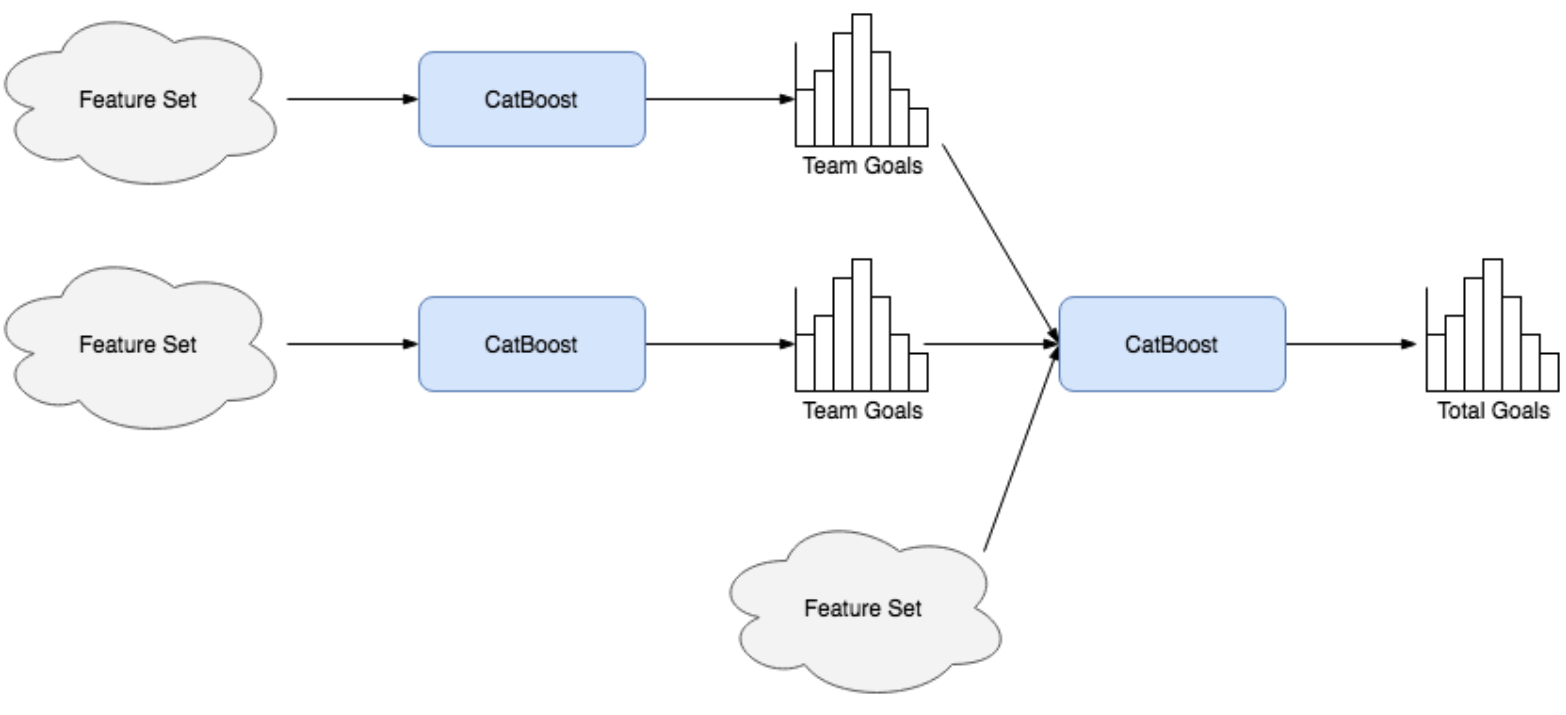
These team-goal models serve as stepping stones towards the sought total. The outputs for either team involved in a game are passed as inputs to a subsequent classifier and supplemented with another feature set containing additional information relating to these teams. Two model types were tested here: a multilayer perceptron and a CatBoost classifier. Once again, the latter performed best.
Two variations of log-loss were used for validation: the same multiclass error used in the team-goal example, and another binary loss using the common 5.5 goals as an over/under total and summing probabilities to give binary likelihoods. Oddly, the multiclass loss was no better than the benchmark – 3.0519 to 3.0515. The binary over/under log-loss, however, beat the benchmark of 0.6847 with a score of 0.6832. We suspect this result is caused in part by nonzero probabilities in goal classes that were absent in the validation data set (there were no instances of 16 or 17 goals). The model also performed poorly on the held-out 2017-18 testing data, scoring a multiclass loss of 3.1271 (benchmark = 3.1240) and a binary log-loss of 0.6967 (benchmark = 0.7022).
Puck Line
The spread was approached in similar fashion to the over/under. By formulating the problem as a multiclassification task, we allow ourselves to easily determine the probability of a game outcome more or less extreme than a given margin of victory (traditionally ±1.5 goals). 24 total classes were used, ranging from 12-goal away team advantage to 12-goal home team advantage. Thus, for a given puck line the suggested probability of beating the spread is simply the sum of probabilities for all outcomes describing a margin of victory greater than the handicap.
As with the over/under, the model output giving probability distributions for team goals were used as inputs. Additionally, the home team’s win probability given by the model described in section 1 and a 48-component feature set were employed. Various neural network architectures were tested but ultimately CatBoost produced the best validation scores. This model’s output was scaled post-prediction such that the sum of probabilities equating to a home team victory were equal to the win probability given by the section 1 model. The validation score was 2.9341 (benchmark = 2.9407) with an accuracy of 26.26% (benchmark = 24.53%). On the held-out 2017-18 season, the model scored 3.0510 (benchmark = 3.0576).
Profitability was evaluated by back-testing the model against Bovada closing odds though the 2017-18 season. Using a simple betting strategy, this model did not generate profit, instead shedding 5.1 units. This disappointing result likely suggests a combination of detracting factors: the predictive model is overfit or poorly constructed, and predicting the margin of victory in NHL games is exceptionally challenging. It is our belief that this model can be greatly improved upon, but it remains unclear whether profitability is attainable. It should also be noted that the model was not tested against opening lines.